Math Model
Part I: Understanding the dynamics of piperamide synthesis
To gain a deep understanding of how a biological system functions, a system of Ordinary Differential Equations (ODEs) offers an excellent approach. Additionally, since we aim to design a novel biosynthetic pathway, modeling the emerging circuit is crucial for deepening our insights and addressing fundamental questions about its behavior.
- What are the inherent limitations of our production system?
- What are the critical steps for optimization?
- Are there alternative, more efficient ways to synthesize our product?
However, every model involves certain assumptions. In this case, we approach the problem using mass-action kinetics, which assumes that enzyme saturation is not a limiting factor. This assumption holds true primarily at low metabolite concentrations. Therefore, our model is a simplification compared to more detailed frameworks like Michaelis-Menten kinetics, which accounts for enzyme saturation. Both mass-action and Michaelis-Menten kinetics can describe dynamic equilibria. For our purposes, this simplification is justified, as we are more concerned with the overall system behavior than the finer details introduced by enzyme saturation.
With that foundation, let’s review our biological challenge:
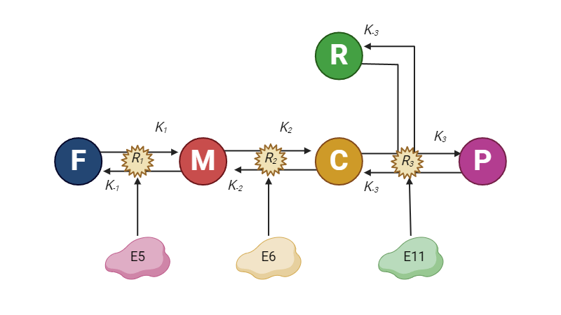
Although our long-term goal is to reproduce the entire pathway for synthesizing piperamide (P), it is relatively cost-effective to simplify the process by introducing Ferulic Acid (F) and Piperidine (R) directly into the medium and expressing only the downstream enzymes. This serves as a substitute for the production of intermediates by the earlier enzymes. In this simplified setup, we focus on just three enzymes: E5, which catalyzes reaction 1, converting F into Methylenedioxycinnamic acid (M); E6, responsible for reaction 2, which converts M into Methylenedioxycinnamoyl-CoA (C); and finally, E11, which facilitates reaction 3, combining C and R to produce Piperamide (P). We assume that these reactions are reversible and governed by specific kinetic constants (K's). Also, we will use a simplified version where the reverse constants are equal to 0.5 while the forward values are 1.
Here comes the algebra
This process can be expressed with a system of ODEs as follows:
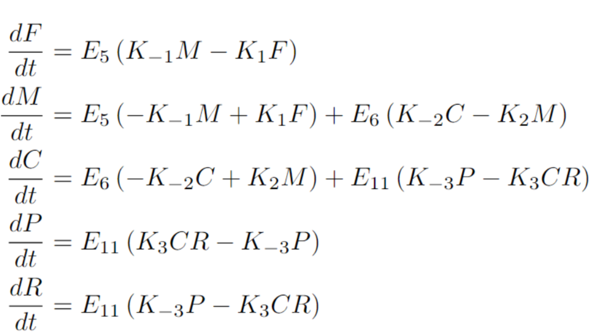
To simplify the model, we will make a couple of key assumptions. First, we assume that the enzyme concentrations for E5, E6, and E11 are identical, which is reasonable since the same promoter drives their expression. Second, we assume that these enzymes have reached equilibrium, meaning their concentrations remain constant rather than dynamic. This assumption holds since we are using a constitutive promoter that has been producing these proteins continuously from the start. To further streamline the system, we normalize by setting the enzyme concentrations equal to one, leaving the dynamics dependent solely on their kinetic constants and the concentrations of the metabolites.
With this system in place, we are now ready to begin exploring the key questions it raises.
Equilibrium behavior
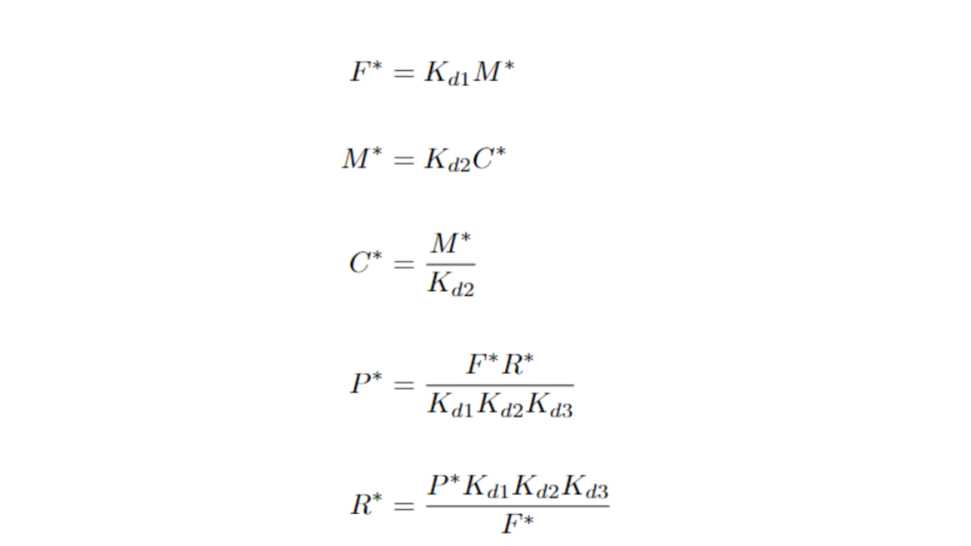
A valuable approach to understanding a system is to identify its equilibrium points. These are the specific combinations of variables (in this case, metabolite concentrations) where there is no net change, meaning the concentrations remain constant over time. Equilibrium points often correspond to attractors, repulsors, or other types of topological structures within the system. To find them, we set each ordinary differential equation (ODE) to zero, indicating no change, and denote the equilibrium state with an asterisk next to the variables.
Upon calculating these points, we observe that our equilibrium points are interdependent, meaning the system lacks a single universal equilibrium point that it consistently converges to. Instead, we encounter an equilibrium surface. For instance, when examining the equation for P*, it becomes clear that the system has as many equilibrium points as multiples of F* and R*—in other words, infinitely many equilibrium points!
We can further explore this idea using a linearization approach. By computing the Jacobian matrix and analyzing its trace (τ) and determinant (Δ) at the equilibrium points, we can interpret the system's topological behavior near equilibrium. This analysis helps us determine the stability and nature of the equilibrium points, such as whether they act as attractors, repulsors, or exhibit more complex dynamics like oscillations. The results are as follows:
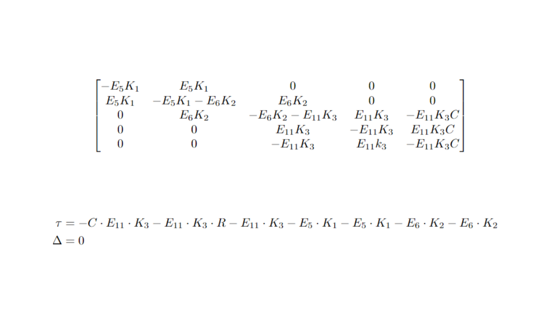
The most significant result is that, since the last two columns of the Jacobian matrix are linearly dependent, its determinant is zero. This indicates that the system does not possess isolated equilibrium points; instead, it features a degenerate node. This topological structure stems from the interdependency of the equilibrium states, supporting the idea that equilibrium can be maintained along a line or surface within the metabolite concentration space.
Moreover, although the node is degenerate, the fact that the trace is negative—since all constants and variables in the model are positive—suggests that the system exhibits stability in certain directions, allowing perturbations to return to equilibrium along those paths.
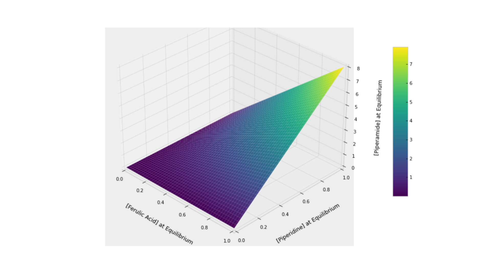
This aligns well with biological expectations in metabolic systems. When a small amount of substrates is added, the system should reach equilibrium, albeit at a lower concentration than if a greater amount had been introduced. In the following figure, we explore this equilibrium surface, showcasing the interaction between Piperidine, Ferulic Acid, and Piperamide, forming a surface that peaks when Piperidine and Ferulic Acid reach their maximum concentrations.
How to interpret equilibrium biologically?
As mentioned earlier, equilibrium refers to a state where there is no change in the variables over time. Biologically, this signifies a balance in metabolic processes, where the rates of production and consumption of metabolites are equal. At equilibrium, the concentrations of the substances involved remain constant, representing a stable condition within the system. In non-engineered biological systems, stability is key for maintaining cellular functions, influenced by factors such as enzyme activity, substrate availability, and feedback mechanisms.
However, our system serves a different purpose: production. Our goal is to maximize the output of piperamide, yet this is biologically constrained by equilibrium, as production will naturally level off after a certain period. Thus, in our context, equilibrium represents the final production yield of piperamide.
With this perspective, we can treat our cells as a function, where the initial concentrations of ferulic acid (F) and piperidine (R) act as inputs (since the concentrations of the other metabolites are initially zero—these compounds cannot be synthesized without the precursors). The cells then "compute" the equilibrium concentration of piperamide (P) for a given combination of F and R. By simulating this system through the integration of our ODEs across various input combinations, we can generate a surface showing that higher initial concentrations of F and R generally yield more piperamide. However, this increase is constrained, as discussed in the "Cytotoxicity" section of our wiki, where we explore the biological limits imposed by other factors.

The resulting surface plot demonstrates the relationship between the initial concentrations of ferulic acid (F) and piperidine (R) and the consequent equilibrium concentration of piperamide (P). The plot reveals a non-linear relationship, where increasing amounts of F and R lead to higher equilibrium levels of P, but with diminishing returns as concentrations approach their maximum. This indicates that while both substrates positively influence piperamide production, the kinetic constraints limit the maximum attainable concentration at equilibrium, forming a curved plateau as shown in the plot.
Part II: What is the most efficient way to produce piperamides?
One day, during lunch, our team started discussing how challenging it would be to engineer a yeast strain capable of reproducing an entire transgenic pathway. Autotoxicity, protein aggregation, pleiotropy, and other issues quickly came to mind—after all, a living organism is an incredibly complex, unpredictable system. Adding more complexity to it would inevitably introduce more problems. We realized that making this project a reality would require years of optimization at every step. Testing our enzymes individually, rather than all together, seemed like the most logical first move. This raised an important question: why not focus on optimizing separate strains using a division of metabolic labor approach?
It suddenly seemed so obvious to us that using a single strain would demand far more effort than splitting the pathway among several strains, each handling a portion of the metabolic workload and transferring metabolites between them. However, we had no idea how efficient such systems could be. Transporting metabolites across the cell membrane posed a particularly tricky challenge, as it limited the amount of metabolites available to each cell.
What if, instead of using multiple cells, we utilized different containers for cell-free systems? This approach would allow us to enjoy the benefits of a simplified system—no membrane barriers, fewer concerns about intracellular interactions, and fewer unpredictable side effects. By eliminating these biological complexities, we could focus purely on optimizing the production of piperamide.
Therefore, before embarking on such a long-term project, we faced a critical question: what is the most efficient way to produce piperamide? Understanding this would be essential for determining whether a cell-free system, multiple or single strains would yield the best results. As we will discuss, we were not sure which one could produce more yield. We initially believed that each could outperform the others for various reasons. However, we ultimately reached the clear conclusion that one was consistently the most efficient.
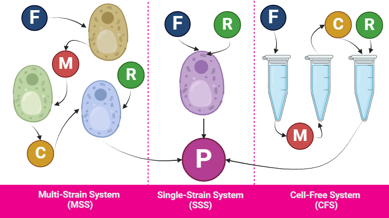
A mathematical model was our initial approach to address this question. Specifically, we developed three distinct yet similar models, one for each alternative.
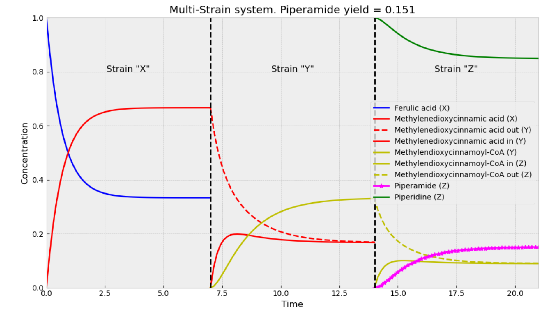
The Single-Strain System (SSS) is the model we previously described. In contrast, for the Multi-Strain System (MSS), we utilized similar equations but decoupled the steps between different enzymes. In this model, we simulated three separate cells, each expressing a different enzyme. When the desired metabolite reached equilibrium in one cell, it was then transferred to the next cell expressing the subsequent enzyme. This necessitated introducing a new type of reaction: across-membrane transport. Consequently, we incorporated additional variables to represent the metabolite concentrations inside and outside the cell. We assumed that the rates of transport into and out of the cell were equal for each metabolite. Finally, piperidine (R) was added as an input to the last medium alongside the previous metabolite (C).
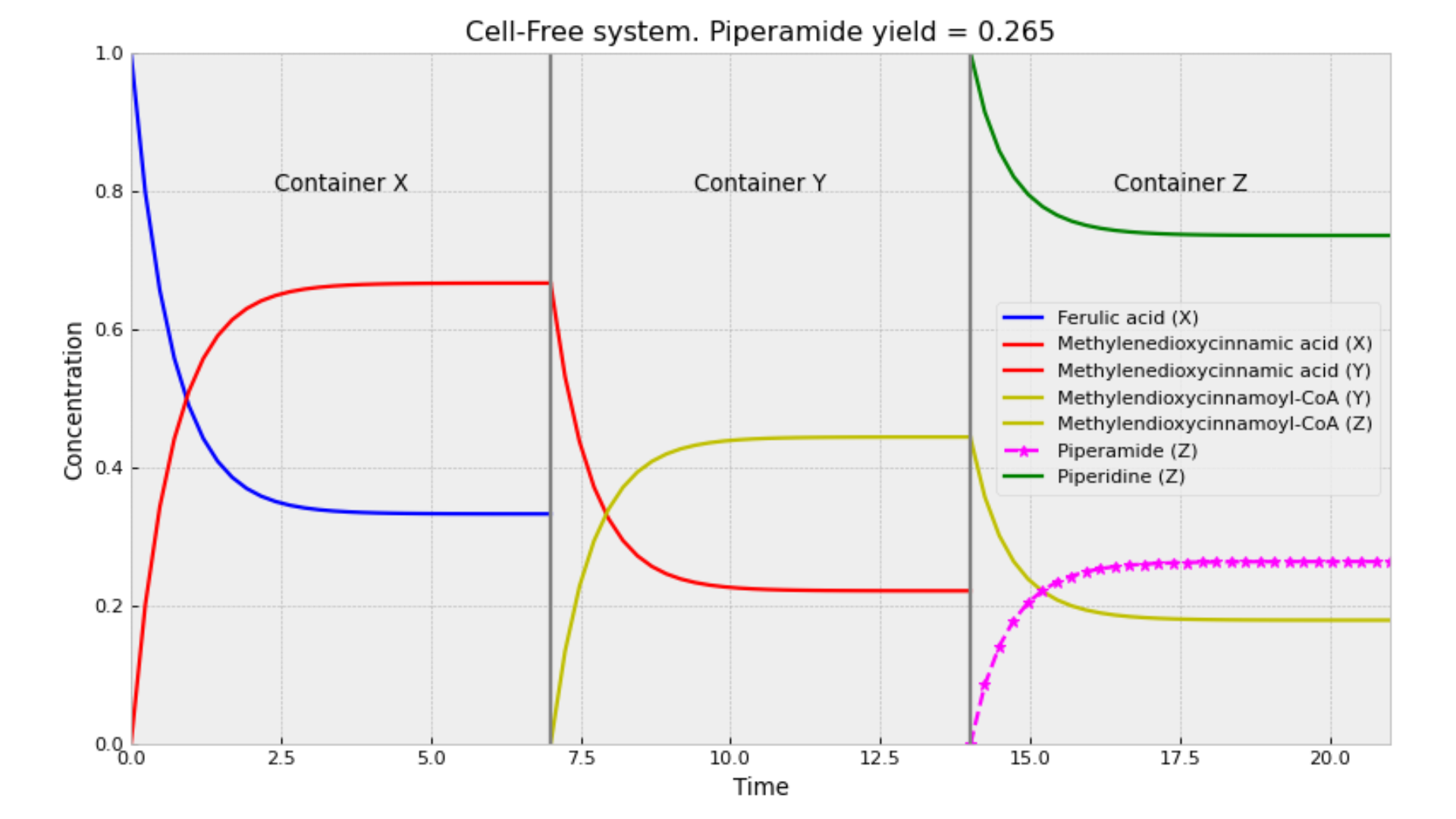
In the case of the compartmentalized Cell-Free System (CFS), we adopted a similar approach, but we did not simulate the concentrations of metabolites inside or outside the system. Instead, three containers substitute the three strains of the MSS.
Multi-Strain Systems are less efficient than Single-Strain Systems
We will use the following equations to prove the stated fact:
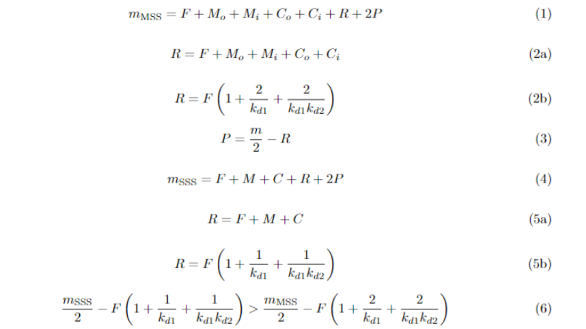
The procedure to demonstrate that the MSS yields less piperamide than the SSS is relatively straightforward. The core concept is based on the principle of mass conservation: since the total mass distributed across metabolites must equal the initial inputs of F and R, we can derive Equation 1. Here, m represents mass, and the subscripts "o" and "i" refer to the "outside the cell" and "inside the cell" compartments, respectively. We use the subscripts MSS and SSS to refer to parameters proper to the corresponding models. Notice that the amount of P is twice the other metabolites, since this balances the fact that two metabolites (C + R) are required to produce a single molecule of piperamide.
It’s important to note that piperamide production requires equal amounts of R∗ and C∗, where C∗ depends on both F∗ and M∗. This relationship is shown in Equation 2a, which establishes that when F∗, M∗, and C∗ reach equilibrium, their combined sum equals R∗. When substituting the equilibrium values for M∗ and C∗ in terms of F∗, we obtain Equation 2b. From 2a, we derive Equation 3, which expresses P∗ (the piperamide concentration at equilibrium) in terms of total mass and R∗. The result indicates that as R∗ increases, P∗ decreases.
A similar approach applies to the SSS. Equation 4 corresponds to Equation 1 in this system, where all metabolites are contained within the cell. Consequently, the equivalent of Equation 2 for the SSS is given by Equation 5. Since Equation 3 is more general, it applies to both systems. However, it becomes clear that Equation 2b yields a larger value for R∗ compared to Equation 5b. Thus, when comparing the substitution of Equation 3 using the values from 2b and 5b, as shown in Inequation 6, it becomes evident that the MSS consistently produces less piperamide than the SSS. However, we treated F as the same amount for both the MSS and SSS, which is incorrect. We will prove in the following section that F is greater for the MSS, thereby concluding this demonstration.
Biologically, this can be interpreted to mean that no matter how efficient the equilibrium points are for each metabolite in the MSS or the nature of their enzyme’s kinetic constants, there will always be a portion of the metabolite that is lost outside the cell. And this loss is always decreasing the maximum yield when compared to the SSS.
Cell-Free Systems are less efficient than Single-Strain Systems
Initially, we strongly believed that compartmentalized CFS would be more efficient than a SSS. When modeling the latter, we observed that increasing the number of metabolites in the pathway decreased the piperamide output. For instance, adding an additional enzyme to produce F caused the equilibrium to distribute across more metabolites, with some mass retained by the new metabolite that would not be used to produce piperamide. Our reasoning was that in a CFS, this wouldn’t be an issue, as each individual container with its respective enzyme would reach maximum equilibrium independently.
However, this assumption was incorrect. To prove this, we will adopt a complementary approach to the previous, in order to demonstrate that the amount of F consumed is greater in the SSS than in the CFS, meaning less F is wasted in the SSS.
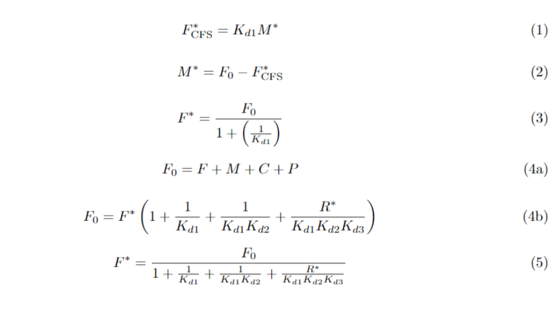
In Equation 1, we depict F at equilibrium in a CFS. Since the first compartment of the CFS contains only one enzyme, just two metabolites—F and M—are involved. M at equilibrium can be expressed in terms of the initial concentration F₀ and the equilibrium concentration of F, as shown in Equation 2. Combining Equations 1 and 2, we derive Equation 3, which expresses F at equilibrium as a fraction of F₀.
In contrast, the mass distribution in the SSS is depicted in Equation 4a. It shows that the initial amount of F is distributed across all metabolites, but their total mass remains constant. At equilibrium, this distribution can be reformulated in terms of F and R, as in Equation 4b. We then arrive at Equation 5, a similar expression to Equation 3, where F is also a fraction of F₀.
When comparing Equation 3 with Equation 5, since the dissociation constants (Kd's) are less than one, and as R*, they are always positive, it becomes evident that the equilibrium concentration of F is lower in the SSS than in the CFS. Thus, the SSS retains less mass in F, using more of it to produce piperamide. The same approach of the previous section can be used here to show that P* is less in the CFS. Similarly, a parallel analysis shows that F is also lower in equilibrium in the MSS, thus completing the previous section’s demonstration.
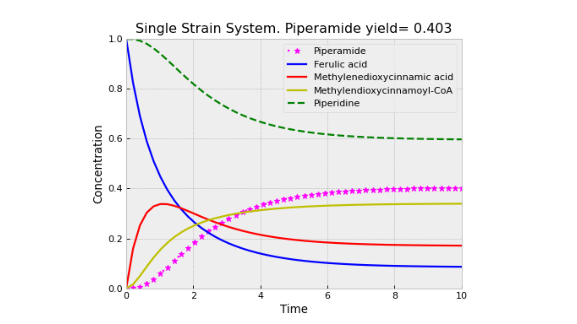
The interpretation of this proof is that in a CFS, the production of M limits the consumption of F, leading to an earlier equilibrium. In contrast, in the SSS, M is consumed as it is produced, which mitigates the limitation on F consumption. In the next figure, it can be seen that a lot of F is retained in the first container.
Also, it is important to consider that this model does not take volumes and diffusion into account, which is the same as assuming that there is a perfect transfer between containers.
Conclusions
The dynamic behavior of piperamide production within a SSS demonstrates several critical characteristics. The system exhibits a stable equilibrium along a surface, allowing for perturbations to return to a steady state, which corresponds to a stable production rate of piperamide. The production efficiency increases as the initial concentrations of ferulic acid (F) and piperidine (R) are raised. However, this result is limited, since the model does not consider enzyme saturation, so a more detailed formulation of the problem could help to better understand the limits of piperamide production.
With the comparison of models and the evidence presented, the following conclusion arises: It is fundamentally impossible to have a more efficient compartmentalization of metabolic labor than the same pathway in a single compartment. The models suggest that the MSS suffers from losses due to the inefficiencies of metabolite transport across cell membranes, and the CFS is limited by the premature equilibrium of intermediate metabolites like methylenedioxycinnamic acid (M), which restricts the use of available ferulic acid (F).
However, while the SSS may be the most efficient model based on our mathematical models, there are several other biological factors that fall outside their scope. These include pleiotropic effects resulting from the expression of multiple enzymes in a single strain, which can lead to unintended interactions and metabolic imbalances. Additionally, the increased metabolite concentration within the SSS can result in autotoxicity, protein aggregation, and metabolic bottlenecks that further complicate scaling up the system. These challenges, along with the inherent unpredictability of biological systems, must be taken into account when designing and optimizing real-world systems for piperamide production. Thus, while SSS is the best approach according to these models, practical considerations require a more holistic view to ensure the system's robustness and efficiency.
As for our project, based on these results, we have chosen to implement a MSS initially. However, our long-term goal is to transition towards a more optimized SSS.